
Visualise the series, deseasonalise it, then test what's left with STL and one or two formal checks. Run the augmented Dickey–Fuller and KPSS tests together to pin down stationarity, add Mann–Kendall to confirm the trend is genuinely monotonic, and save Bayesian or change-point models for cases involving regime shifts or where you need honest uncertainty bounds. That order matters more than the specific test you pick.
TL;DR:
- Deseasonalising with STL before testing is crucial, as unaddressed seasonality can mask or falsely indicate trends.
- Combining tests like ADF, KPSS, and Mann–Kendall provides more reliable trend detection and helps resolve conflicting results.
- Sensitivity analysis on parameters such as smoothing window or trend velocity prevents false trend identification caused by small variations.
- Bayesian trend models and change-point detection are essential for identifying regime shifts or structural changes over time.
- Automated AI pipelines with cross-checked outputs improve scale and reliability in noisy, evolving markets compared to manual analysis.
Table of Contents
- What counts as a trend in time series trend detection
- Comparing methods for time series trend analysis
- A step-by-step workflow for trend detection
- Advanced approaches for regime shifts and evolving dynamics
- How Ontherice tackles trend detection in noisy market data
- Judging whether a trend detection method actually works
- Handling non-stationarity before it wrecks your forecast
- Where trend detection earns its keep in practice
- Why trend detection still trips up experienced analysts
- Practitioner pitfalls worth avoiding
- Put this workflow to work with Ontherice
- Sources
What counts as a trend in time series trend detection
A trend is the long-run direction of a series once you strip away the noise. The trend-cycle component (the combined smooth movement, including slow business-cycle swings) is what most analysts mean when they say "trend," because pure trend and cycle rarely separate cleanly in practice.
Seasonality and cycles get confused constantly, and the distinction changes which method you should reach for. Seasonality repeats at a fixed, known frequency, such as weekly retail spikes or December sales surges. A cycle has no fixed length; a business cycle might run several years, and you only know its shape in retrospect. This distinction, laid out clearly in Forecasting: Principles and Practice, decides whether you can even use seasonal-adjustment tools at all.
Decomposition splits a series into trend, seasonal, and remainder components, and the choice between additive and multiplicative structure depends on how the fluctuations behave:
- Additive decomposition fits when seasonal or trend-cycle swings stay roughly constant in size regardless of the series' level.
- Multiplicative decomposition fits when those swings scale up as the series grows, which is common in some economic or demographic data.
- When multiplicative behaviour shows up but your tools assume additive structure, log-transform the data first rather than switching frameworks entirely.
Skipping decomposition before testing is the single most common error analysts make: unaddressed seasonality can mask a real trend or fake one that isn't there.
Comparing methods for time series trend analysis
Every trend-detection method makes a trade-off between smoothness, sensitivity to outliers, and how much data it demands. None of them wins outright. The job is matching the tool to your data's frequency and your tolerance for false positives.
Smoothing and filtering approaches:
- Simple moving average: cheap and transparent, but lags badly at turning points and needs a clean, evenly spaced series.
- EWMA (exponentially weighted moving average): reacts faster than a moving average because recent points carry more weight; the smoothing parameter (alpha) trades responsiveness against noise, and it roughly maps to an equivalent moving-average window (a smaller alpha behaves like a longer window).
- STL/LOESS decomposition: the most flexible option for separating trend from seasonality, and it copes well with changing seasonal patterns. It is robust to missing values and outliers but requires you to set smoother-length parameters correctly.
- Hodrick–Prescott (HP) filter: isolates a smooth long-run trend by penalising curvature, popular in economics, but it's known to distort estimates near the edges of the sample and can manufacture spurious cycles if the smoothing parameter is misjudged.
- Kalman smoother: handles time-varying trends elegantly and copes with missing data, at the cost of requiring a state-space model specification upfront.
Formal statistical tests:
The augmented Dickey–Fuller (ADF) test checks for a unit root, meaning it tests the null hypothesis that the series is non-stationary. The KPSS test does the reverse, testing the null hypothesis that the series is stationary. Because they test opposite nulls, running both together is standard practice, and when they disagree (ADF says stationary, KPSS says non-stationary, or vice versa) it usually signals a series that's stationary around a trend rather than cleanly one or the other.
Statistic to know: STL's own documentation recommends setting the trend smoother length to about 1.5 times the seasonal smoother length, and the seasonal window should be an odd number, or the decomposition biases the trend estimate. See statsmodels STL docs.
For monotonic trends without assuming normality, the Mann–Kendall test is the workhorse. It's non-parametric and robust to outliers, which makes it a better first choice than a linear regression slope test when your data is messy or skewed, common in environmental and sensor data.
A step-by-step workflow for trend detection
Skipping steps here is how analysts end up trusting a trend that's actually seasonal noise in disguise. Work through this sequence rather than jumping straight to a test.
- Plot the raw series first. A line plot, a seasonal subseries plot, and the ACF/PACF together tell you more in five minutes than any single statistic. Look for changing variance, missing chunks, and obvious seasonal repetition.
- Preprocess and deseasonalise. Handle missing values honestly (don't just interpolate blindly), and if variance grows with the level of the series, log-transform before anything else. Remove seasonality if it's present, using STL rather than a naïve seasonal average.
- Extract the trend and run your tests. Apply STL alongside a second method (an HP filter or the trendseries package in R, which wraps HP, Baxter-King, Christiano-Fitzgerald, STL, LOESS, and Kalman filters behind one interface). Run ADF and KPSS on the deseasonalised series, then Mann–Kendall to confirm monotonic direction.
- Quantify trend velocity. Fit a local linear model over a rolling window and track the slope, this is your trend velocity metric. Then check how sensitive that slope is to your choice of window length or smoothing parameter; a trend that vanishes when you nudge the window by 10% isn't a trend you should act on.
- Validate against forecasting performance. Does including the extracted trend actually improve out-of-sample forecast accuracy? Backtest across the series looking for structural breaks the trend model might be papering over.
Pro Tip: Always inspect the trend-cycle component directly when hunting for turning points, not the seasonally adjusted series. Seasonally adjusted data still carries the remainder term, which can produce jagged, misleading "turns" that aren't there in the actual trend.
Advanced approaches for regime shifts and evolving dynamics
Standard filters assume the trend behaves consistently. When it doesn't, when a market shifts regime overnight or a slow structural change unfolds over years, you need tools built for that instability, at a real computational cost.
- Bayesian trend models put priors on the smoothness of the trend and return full posterior uncertainty rather than a single point estimate. They suit gradual, evolving shifts where you need to communicate confidence intervals to a decision-maker, not just a slope.
- Change-point detection flags sudden regime breaks rather than gradual drift. Offline detectors scan the whole series retrospectively and find breaks with high precision; online detectors flag breaks as new data arrives but trade some accuracy for lower detection latency, an important distinction if you're monitoring live data feeds.
- Time-varying autoregressive (TVAR) and state-space Unobserved Components models let the trend's own dynamics evolve smoothly over time rather than assuming a fixed structure, useful for series where the "normal" growth rate itself is drifting.
These methods generally need longer histories, more careful setup, and more computing time than STL or a moving average. Flexible approaches like these trade simplicity for the ability to quantify uncertainty properly, which matters when the trend estimate feeds directly into a costed decision. The sensible default is running a simple filter first and escalating to Bayesian or change-point methods only when the simple approach visibly fails, sudden jumps it can't explain, or residuals that refuse to look like noise.
How Ontherice tackles trend detection in noisy market data
The problems above (seasonality masking direction, single tests giving false confidence, regime shifts breaking simple filters) are exactly what Ontherice's detection pipeline is built to handle at scale, across markets that never sit still.
- The platform runs multiple AI engines in parallel over global public data, rather than relying on one model's read of a noisy signal.
- Cross-checking outputs across engines works similarly to triangulating ADF, KPSS, and Mann–Kendall by hand: agreement across independent methods cuts down false positives that a single test would miss.
- Rankings and scores are published with a visible history so that a signal's track record is checkable rather than asserted.
- The platform's pipeline approach to AI trend detection treats extraction as a chain of checks, not a single model output, mirroring the workflow discipline this article has walked through.
Transparent ranking history matters here precisely because trend detection is probabilistic, not certain. A system that shows its track record, rather than just its current call, gives you something to actually evaluate.
Judging whether a trend detection method actually works
A trend model that looks elegant on a chart and fails on new data is worse than no model at all, so evaluation has to go beyond visual inspection.
Out-of-sample forecast accuracy is the most honest test: does adding your extracted trend to a forecasting model reduce error (RMSE, MAE, or MAPE, depending on your series' scale) on data the model never saw during fitting? A trend that fits history beautifully but doesn't improve forecasts is describing the past, not predicting the future.
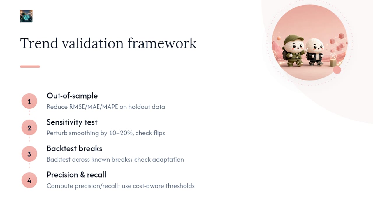
Sensitivity analysis matters just as much as accuracy. Perturb your smoothing window by 10 or 20% and rerun the extraction. If the trend direction or velocity flips under a small parameter change, the signal is fragile, not real. This is where a lot of published "trend discoveries" quietly fall apart under scrutiny.
Backtesting for structural breaks checks whether your trend model would have caught, or missed, past regime shifts. Run the pipeline on a historical window ending before a known break and see whether it adapted sensibly afterward or kept extrapolating the old direction.
For classification-style trend labelling (up, neutral, down), precision and recall against a labelled test set apply directly, and some quantitative finance pipelines go further, incorporating transaction-cost-aware thresholds so a "detected" trend only counts if it would have been profitable to act on, not just statistically present. That's a meaningfully higher bar than pure statistical significance, and it's the right one when a trend call feeds directly into a spending or trading decision.
Handling non-stationarity before it wrecks your forecast
Non-stationary data breaks the assumptions behind most classical forecasting models, and detrending is the usual fix, but it comes with a catch. If your ADF and KPSS results confirm a unit root, you typically need to difference the series or extract the trend explicitly before feeding it into an ARIMA-style model or a regression.
The catch is this: aggressive detrending can strip out exactly the signal you were trying to forecast. Over-differencing a series that only has a mild drift can leave you modelling pure noise, while under-differencing leaves residual trend contaminating your error terms and invalidating confidence intervals. This is why running ADF and KPSS together matters so much; relying on ADF alone can lead you to difference a series that KPSS would have flagged as already stationary around a deterministic trend, a different problem requiring a different fix (detrending, not differencing).

For forecasting specifically, the practical implication is this: a trend extracted via STL or an HP filter should be added back into the forecast after the deseasonalised, detrended component has been modelled, not discarded. The trend is information, not junk to be cleaned away. Getting this sequencing wrong, differencing when you should detrend, or detrending when you should difference, is one of the more common reasons a technically correct model still produces forecasts that drift systematically off target within a few periods.
Where trend detection earns its keep in practice
Central banks and statistical agencies run trend-cycle extraction on GDP and employment data every month specifically to separate genuine turning points from seasonal noise, which is why headline "seasonally adjusted" figures get revised as more data arrives and the trend estimate stabilises.
In retail and e-commerce, Mann–Kendall-style monotonic trend tests on deseasonalised sales data help distinguish a genuine growth trend from a temporary seasonal peak, the difference between restocking for sustained demand and over-ordering for a spike that's about to reverse.
Environmental science leans heavily on Mann–Kendall precisely because of its robustness to non-normal data and outliers, applied to river flow records, temperature series, and pollutant concentrations where a handful of extreme readings shouldn't be allowed to dictate the conclusion.
In markets and finance, change-point detection flags regime shifts, a volatility spike, a policy shock, faster than a slow-moving average ever could, while HP-filtered or Kalman-smoothed trend estimates feed into longer-horizon strategic positioning where reacting to every daily wiggle would be counterproductive. The common thread across all four domains: the method choice tracks the decision it feeds, fast-reacting change-point detectors for tactical calls, smooth long-run filters for strategic ones.
Why trend detection still trips up experienced analysts
Non-stationary, noisy real-world data rarely matches the tidy assumptions behind these methods, and the gap between textbook and dataset is where most errors creep in.
Outliers and structural breaks distort smoothing filters silently. An HP filter fed a series with an unaddressed one-off shock (a supply disruption, a policy change) will bake that shock into its trend estimate rather than isolating it, because the filter has no way to distinguish a permanent shift from transient noise unless you tell it to.
Short series create real limits. STL, Kalman smoothers, and Bayesian trend models all want enough history to estimate their parameters reliably. With only a year or two of monthly data, seasonal decomposition becomes unstable, and confidence in any extracted trend should shrink accordingly.
Parameter choices are underappreciated leverage points. The STL seasonal window, the HP filter's smoothing constant, the EWMA alpha, small changes here can flip a "rising" trend into a "flat" one. Few analysts run the sensitivity checks that would catch this before publishing a conclusion.
Contradictory test results get resolved badly. When ADF and KPSS disagree, the temptation is to pick whichever result supports the story you already wanted to tell. Treat disagreement as information about the series' structure, not noise to explain away.
Multiple valid answers exist simultaneously. HP and Hamilton filters, for instance, return genuinely different notions of trend, a smooth long-run path versus a business-cycle deviation, and neither is wrong. The error is assuming there's one true trend waiting to be found rather than a family of reasonable estimates depending on what question you're actually asking.
Practitioner pitfalls worth avoiding
Deseasonalised data is not the same as clean data. Always inspect the residual component separately from the trend-cycle. A tidy-looking deseasonalised chart can still be hiding a jagged remainder that's driving false turning-point signals.
Never call a trend, or a stationary series, off one test. Triangulate ADF, KPSS, and Mann–Kendall, and treat disagreement as a signal about series structure rather than a nuisance to override.
When a trend call carries real cost (a trade, a stocking decision), run sensitivity analysis and consider cost-aware thresholding rather than a simple binary up-or-down label. The temporal trends feeding market decisions that actually pay off are the ones stress-tested before anyone acts on them.
— Aidil
Put this workflow to work with Ontherice
This platform is built for similar bottlenecks: running STL, stationarity checks, and trend velocity tracking manually across dozens of markets doesn't scale, but a multi-engine AI pipeline scanning global data continuously does. Instead of building your own detection stack from scratch, you get real-time extraction, transparent rankings, and a visible accuracy history you can check against, rather than take on faith.

If you want a live read on where signals are building before they're obvious, the AIOpportunities feed surfaces early AI-selected trends across finance, products, crypto, and jobs. Readers who want the methodology behind the ranking system before committing can work through the Ontherice whitepaper first, and those who want to see the engines themselves can explore the AiTools page. Start with the AIOpportunities feed and see what your market's trend velocity actually looks like this week.
Sources
For hands-on implementation, the canonical references are worth bookmarking directly:
- Forecasting: Principles and Practice (OTexts) — components
- trendseries: Extract Trends from Time Series — CRAN