TL;DR:
- Temporal trends carry crucial information that influences sound business strategies, but are often overlooked or misinterpreted. Recognizing trend shapes, properly adjusting for seasonality, and analyzing epoch-based periods prevent costly analytical errors and misleading conclusions. Implementing time-aware models and developing temporal literacy are essential for making accurate forecasts and better organizational decisions.
Understanding the role of temporal trends is one of the most underrated skills in business analysis, yet it is where the most costly mistakes happen. Analysts who treat time as a backdrop rather than an active variable routinely draw conclusions that are statistically convincing and practically wrong. A rising metric in your data might reflect genuine structural growth, a seasonal blip, or the tail end of a shock that started years before you started measuring. The difference between those three interpretations is the difference between a sound strategy and an expensive miscalculation.
Table of Contents
- Key takeaways
- Understanding the role of temporal trends
- Statistical pitfalls: spurious results and seasonal distortion
- The impact of temporal trends on business decisions
- Tools and techniques for temporal trend analysis
- My perspective: why most analysts still get this wrong
- Discover temporal intelligence with Ontherice
- FAQ
Key takeaways
| Point | Details |
|---|---|
| Temporal trends vary in shape | Trends can be stable, linear, or quadratic; fitting a single line across all data obscures the real signal. |
| Seasonality masks true signals | Removing seasonal and calendar effects is necessary before comparing periods or drawing economic conclusions. |
| Spurious results are a real risk | Ignoring non-stationarity in time series produces misleading correlations that appear statistically significant. |
| Business cycles are compressing | Faster decision cadences require shorter sensing-to-action loops, making continuous trend monitoring a priority. |
| AI improves temporal analysis | Time-aware models consistently outperform standard approaches when predicting outcomes from longitudinal data. |
Understanding the role of temporal trends
Time is not a neutral dimension in data. It shapes every metric you track, and the pattern that data traces over time carries information that a single snapshot cannot. A temporal trend is the underlying direction a variable moves across a period, after you account for random variation, seasonality, and one-off shocks. The importance of time trends lies precisely in that definition: you cannot see the true direction without first removing everything else.
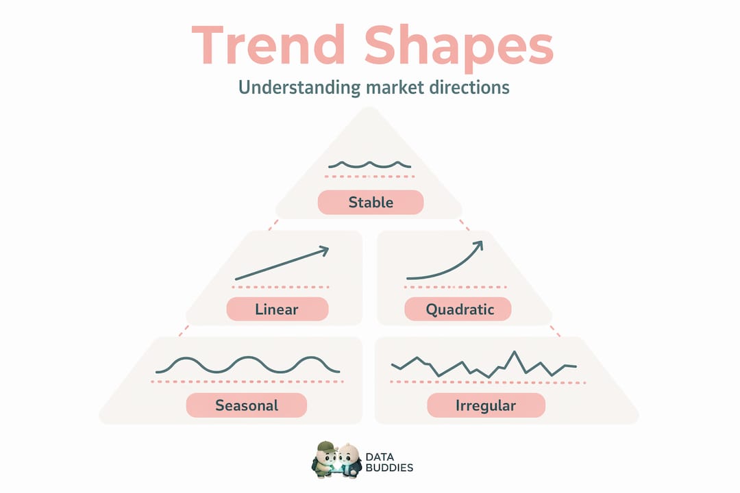
There are three core shapes a temporal trend can take. A stable trend shows no meaningful change over the observation period. A linear trend moves at a consistent rate in one direction. A quadratic trend accelerates or decelerates, curving upward or downward over time. Distinguishing between them matters far more than most analysts assume. Research tracking 31,411 pregnancies across pre-pandemic, lockdown, and post-restriction periods found that different outcome measures followed stable, linear, and quadratic trajectories simultaneously within the same dataset.
Velocity is a concept worth adopting explicitly. Rather than simply noting "the trend is upward," velocity quantifies the annual absolute change, giving you a rate rather than a direction. A large study spanning 232 million participants from 1980 to 2024 used velocity to map global obesity dynamics, revealing that some high-income countries have plateaued while others continue to accelerate. That distinction is invisible if you only look at the direction of the trend.
Pro Tip: Avoid fitting a single linear model across an entire dataset. Divide your observation window into epochs and test whether the trend shape changes across them. A flat early period followed by a steep rise is not the same as a consistent upward slope, even if the endpoint looks identical.
Understanding temporal patterns also means recognising that trends are rarely global across an entire dataset. Epoch-based decomposition, where you model each sub-period separately, produces far more accurate descriptions of what is actually happening and why. This approach is explained in more detail in Ontherice's guide to trend lifecycle analysis for analysts who want a structured framework.
Statistical pitfalls: spurious results and seasonal distortion
The most common error in time series analysis is not a calculation mistake. It is a modelling assumption: treating data as if time does not matter. When you run a regression on two variables that both trend over time, the model can find a statistically significant relationship between them that has no causal basis whatsoever. This is called a spurious regression, and it is far more common in business reporting than anyone is comfortable admitting.
A textbook example comes from inflation and unemployment data: regressing one against the other without controlling for the time trend produces a coefficient that contradicts economic theory entirely. The variables look related because they both trend over time, not because they influence each other. Econometric best practice distinguishes between deterministic and stochastic trends, each requiring a different correction. Deterministic trends are handled by including a time variable directly in the model. Stochastic trends require differencing or unit root testing, and simply adding a time variable is not sufficient.
Seasonality introduces a separate but equally damaging distortion. Monthly retail figures always rise in December. Quarterly employment numbers shift predictably with the academic year. These are not signals. They are calendar artefacts, and treating them as signals leads to the wrong conclusions. Seasonal adjustment removes these predictable effects to clarify the underlying economic movement, using methods such as X-12-ARIMA to produce period-to-period comparisons that are actually meaningful.
The practical implication is clear. Canada's seasonally adjusted Transportation and Supply Chain Index surpassed December 2019 levels from October 2021 onward, something the raw monthly figures would have obscured beneath predictable seasonal fluctuation. Without adjustment, the recovery story is blurred.
Pro Tip: Before building any model on time-series data, run a stationarity test such as the Augmented Dickey-Fuller test. If your data is non-stationary, differencing or detrending is not optional. Skipping this step makes every coefficient in your model unreliable.
The broader principle here: failing to control for non-stationarity causes systematically biased inference. This is not a technical nicety. It is the difference between a forecast that guides decisions and one that misleads them.
The impact of temporal trends on business decisions
Understanding temporal patterns at a technical level only matters if it changes what you decide. The impact of temporal trends on real business outcomes is substantial and often underappreciated.

Consider demand forecasting. A retailer who observes a steady sales climb over twelve months might plan aggressive inventory expansion. But if that trend is driven by a quadratic acceleration that is already decelerating, the peak has passed by the time the stock arrives. Accurate trend-shape analysis prevents exactly that kind of costly misread. This is why AI-driven trend discovery has become a competitive differentiator rather than a nice-to-have.
Pandemic-era data reinforced this lesson sharply. Many analysts attributed dramatic shifts in health and economic indicators to COVID-19 as a discrete shock. Research examining pregnancy outcomes during this period found that many apparent pandemic-related changes were actually continuations of pre-existing trends, not new phenomena. The shock reframing was wrong because analysts had not modelled the pre-pandemic trajectory carefully enough to recognise continuity when they saw it.
The following table illustrates how different trend types translate into different strategic demands:
| Trend type | Characteristic behaviour | Strategic implication |
|---|---|---|
| Stable | Metric holds within a narrow band over time | Optimise costs and maintain current positioning; no growth urgency |
| Linear | Consistent directional movement at a steady rate | Plan capacity and resources in proportion to the rate of change |
| Quadratic (accelerating) | Rate of change itself is increasing | Act early; the window before competitors notice is narrow |
| Quadratic (decelerating) | Growth or decline is slowing toward plateau | Avoid overcommitting to projections built on earlier velocity |
| Heterogeneous | Different sub-markets show different trend shapes simultaneously | Segment analysis before drawing any aggregate conclusion |
How do temporal trends affect outcomes in organisational strategy? 70% of business leaders now report that they need to balance stability with agility, driven by faster decision cadences. Compressed business cycles demand shorter sensing-to-decision loops, and that is only achievable if your trend analysis is running continuously, not in quarterly review cycles.
Tools and techniques for temporal trend analysis
Knowing what can go wrong with temporal data is half the picture. The other half is having practical techniques to do it correctly. The decomposition framework is the most transferable starting point.
Any observed time series can be broken into four components:
- Trend-cycle: the long-run direction of the series, smoothed of short-term fluctuation
- Seasonal: predictable, repeating patterns tied to the calendar
- Calendar effects: irregular but predictable factors like trading-day variation or holidays
- Irregular: what remains after removing the above three, representing genuine noise or unexplained shocks
Generalised additive models (GAMs) offer a flexible way to model trend-cycle components without forcing a linear assumption. They allow the trend to curve, flatten, and shift direction across epochs, which is precisely what most real-world business data does. This flexibility is particularly useful when you suspect a trend has changed shape partway through your observation window, as flexible GAM approaches have demonstrated in clinical and public health data contexts.
For analysts working with machine learning pipelines, the ordering of observations is not just metadata. Time-aware frameworks for longitudinal data consistently achieve higher predictive accuracy than models that treat observations as exchangeable. A model that learns which features matter at which point in a sequence is simply a better model for any time-indexed problem.
Choosing the right observation window is also a practical decision that deserves deliberate thought. Trends measured over three years can look entirely different from trends measured over ten, particularly if a structural shift occurred midway. Ontherice's step-by-step forecasting guide covers window selection as part of a structured approach to business forecasting.
My perspective: why most analysts still get this wrong
I've spent years watching analysts, including experienced ones, treat temporal trends as background detail rather than foreground signal. The pattern is consistent: the model gets built, the results look reasonable, and nobody asks whether the time dimension was handled properly. The results get presented. Decisions get made. And the miscalibration only becomes visible six or twelve months later when reality diverges from the forecast.
What I've found is that the problem is not usually a lack of technical knowledge. Most analysts know what stationarity is. The problem is a cultural one. There is institutional pressure to produce clear, confident findings quickly, and proper temporal modelling takes time and produces nuance. "The trend is upward but decelerating and the shape varies by segment" is a harder message to sell than "the trend is upward."
The rise of compressed decision cycles has made this worse, not better. Faster feedback loops are only valuable if the signals feeding them are properly adjusted for seasonality and trend shape. Speed without accuracy amplifies errors rather than correcting them.
My view is that temporal literacy needs to be treated as a core analytical skill at the same level as statistical literacy. That means training analysts to decompose data before modelling it, to test for stationarity as a default step, and to question whether what looks like a recent shift is really a pre-existing trajectory that was never properly characterised. The organisations doing this well are not simply getting better forecasts. They are making structurally better decisions. You can read more about how trends shape strategic planning and why this matters at an organisational level.
— Aidil
Discover temporal intelligence with Ontherice
If you are tracking markets where trend shapes matter, whether that is supply chain signals, sector momentum, or emerging B2B demand patterns, the tools you use need to be built for temporal complexity, not just aggregate volume.

Ontherice is built precisely for this. Its AI engines scan global data continuously, separating real signals from noise by factoring in time-sensitive dynamics that standard analytics tools miss. B2BSignals gives you a live view of evolving business signals before they reach consensus awareness. AIOpportunities surfaces market trends that are accelerating, not just large. And the RankingsGeneratorEngine produces dynamic, time-aware rankings across sectors so you can track which opportunities are gaining velocity right now. When the difference between a quadratic acceleration and a plateau determines your next move, Ontherice gives you the temporal precision to act with confidence.
FAQ
What is the role of temporal trends in data analysis?
Temporal trends reveal the underlying direction of a variable over time, after accounting for seasonality, noise, and one-off shocks. Correctly identifying the trend shape, whether stable, linear, or quadratic, determines whether analytical conclusions are reliable or misleading.
How do temporal trends affect business forecasting?
Trend shape directly influences demand projections and resource planning. A decelerating quadratic trend requires very different inventory and capacity decisions than a linear one, even if both show an upward movement over the observation period.
Why does ignoring seasonality cause problems?
Seasonal patterns are predictable and repeat on a calendar cycle, so leaving them in your data makes period-to-period comparisons unreliable. Analysts who skip seasonal adjustment can misread routine fluctuations as structural changes, leading to poor strategic calls.
What is a spurious regression in time series analysis?
A spurious regression occurs when two variables both trend over time and appear statistically related in a model, even though no genuine relationship exists. Controlling for non-stationarity through differencing or detrending is the standard corrective.
How can AI improve the analysis of temporal trends in data?
Time-aware AI models incorporate the ordering and spacing of observations, which standard models ignore. Research shows that these frameworks achieve measurably higher predictive accuracy on longitudinal datasets, making them a practical upgrade for any analyst working with time-indexed business data.