
Time series anomaly detection means learning what "normal" looks like in sequential data, and then flagging points or windows that deviate from it. The practical verdict: model normal behaviour with a forecasting or reconstruction approach, score the residuals or reconstruction error, and apply dynamic rather than fixed thresholding. Prediction-based methods suit stable, seasonal signals; reconstruction suits noisy multivariate telemetry; representation-based methods suit sparse labels.
TL;DR:
- Prioritize simple, statistical baselines like STL decomposition and exponential smoothing before deploying neural network models.
- Use dynamic, nonparametric thresholding for alerts, as it adapts better to drifting data and reduces false positives.
- Combine forecasting and reconstruction methods with lightweight ensemble approaches for more operationally relevant anomalies.
- Validate anomaly detection systems with range-based metrics and synthetic anomalies to ensure real-world effectiveness.
- Expect generative models to enhance training with synthetic anomalies but treat new architectures as hypotheses to test against your own data.
Table of Contents
- What are the main families of time series anomaly detection methods?
- Which algorithms actually work for time series anomaly detection?
- How do you build a practical time series anomaly detection pipeline?
- How should you evaluate a time series anomaly detector?
- What's next for time series anomaly detection research?
- Why simple pipelines still beat clever models
- Sources
What are the main families of time series anomaly detection methods?
Every detector, however sophisticated, falls into one of five families, and the choice depends more on your data regime than on model fashion. A decade-spanning survey of time series anomaly detection makes this explicit: no single detector wins across heterogeneous datasets, so matching the family to the data matters more than chasing the newest architecture.
- Distance-based methods flag points far from their nearest neighbours in a windowed embedding space. They are good for low-dimensional, low-noise signals but weak on high-dimensional or highly seasonal data.
- Density-based methods (local outlier factor and relatives) look for sparse regions in feature space. Useful when anomalies cluster loosely rather than sitting as isolated spikes.
- Prediction-based methods forecast the next value and score the gap between forecast and actual. Best when the series has strong temporal structure and enough history to learn it.
- Reconstruction-based methods compress and rebuild the input; large reconstruction error signals an anomaly. Suited to multivariate, noisy sensor data where no single feature carries the whole signal.
- Representation-based methods learn general embeddings (often self-supervised) and detect anomalies as embedding-space outliers. Useful with scarce labels or when transferring across related series.
A conference tutorial on deep TSAD methods groups deep-learning techniques specifically into forecasting, reconstruction and representation approaches, each carrying different assumptions about how much "normal" data you need and whether labels exist at all.
Which algorithms actually work for time series anomaly detection?
Start simple. Classical decomposition and smoothing methods remain the fastest way to separate trend, seasonality and residual noise, and engineering guides consistently recommend running these baselines first before reaching for anything heavier.
- Statistical baselines: STL decomposition, exponential smoothing and ARIMA residuals catch seasonal and trend anomalies cheaply, and give you an interpretable benchmark everything else must beat.
- Isolation and proximity methods: isolation forest variants partition the feature space randomly and isolate outliers in fewer splits. They scale well to high-dimensional, streaming settings, which is why surveys on isolation mechanisms highlight their low memory footprint for production telemetry.
- Forecasting models: ARIMA, gradient-boosted regressors, or LSTM networks predict the next step; the prediction error becomes your anomaly score. LSTMs handle longer dependencies but need more data and tuning than a simple regressor.
- Reconstruction models: autoencoders, variational autoencoders and GANs learn to compress and rebuild normal sequences. When reconstruction fails badly, that failure is the anomaly signal, and generative approaches are increasingly extending this toward diffusion-based architectures.
- Transformers and representation methods: self-attention captures long-range dependencies transformers excel at, but they demand more compute and more careful interpretability work than simpler models.
Pro Tip: Run a statistical baseline and an isolation-based model before touching a neural network. If both catch the anomalies your stakeholders care about, you have saved weeks of tuning.
How do you build a practical time series anomaly detection pipeline?
Every reliable pipeline follows the same skeleton, whatever model sits inside it. Get the plumbing right and even a modest model performs well; get it wrong and the best architecture won't save you.
Start with data checks: resample to a consistent frequency, decide how to handle missing values (interpolation for short gaps, masking for long ones), and identify seasonal cycles before modelling. For multivariate data, windowing choices (window length, stride, overlap) shape what "context" the model sees, and feature engineering (rolling statistics, lag features, frequency-domain transforms) often matters more than model choice.
Pick your learning regime deliberately:
- Unsupervised when you have no labelled anomalies, which describes most production telemetry.
- Semi-supervised when you have confirmed normal data and want the model to flag deviations from it.
- Supervised only when you have enough labelled anomalies to justify the cost, which is rare outside finance and fraud.
Post-processing decides whether your alerts are useful or ignored. Smoothing raw error scores, aggregating across sensors, and pruning short-lived spikes cuts noise substantially. Static thresholds break down the moment your data drifts, which is why work on spacecraft telemetry introduced dynamic, nonparametric error thresholding that adapts to non-stationary error distributions and materially cuts false positives compared with fixed cut-offs.
In practice: teams that pair a modest forecasting model with adaptive thresholding routinely outperform teams running a more complex model on a static cut-off, because the threshold logic is doing most of the precision work. For deployment, track inference latency against your alerting SLA, monitor for concept drift with a rolling retraining cadence, and route flagged alerts through a human triage step before they reach operators. Ontherice's own trend detection validation checklist is a useful reference for structuring that validation step.
How should you evaluate a time series anomaly detector?
Point-wise metrics lie to you. A detector that fires one timestep late on every genuine anomaly scores badly on strict point-wise precision and recall, even though it is operationally useful, which is exactly why range-based metrics exist.
- Point vs range-based metrics: point metrics judge exact timestamp matches; range-aware metrics credit a detector for overlapping the true anomalous interval, which better reflects real alerting behaviour.
- Precision, recall and F1 remain the baseline reporting trio, but always state whether they are point-wise or range-adjusted.
- AUC and VUS (volume under the surface) extend evaluation across multiple threshold and tolerance settings simultaneously, reducing the risk of cherry-picking one favourable operating point.
- Protocol discipline: use temporal holdout splits (never shuffle time series randomly), inject synthetic anomalies to test recall on known events, and report your exact thresholding method so results are reproducible.
Benchmarking is where most published comparisons quietly mislead readers. A VLDB tutorial on TSAD trends points out that mislabelled ground truth, skewed anomaly rates and inconsistent metric choices routinely distort published leaderboards, and that no single detector wins consistently across benchmark datasets. The practical fix is mundane but effective: build your own small labelled validation slice from real incidents rather than trusting public benchmark rankings alone, and consider tools that evaluate trend proxies rather than raw accuracy figures, as Ontherice's proxy evaluation guide discusses.
What's next for time series anomaly detection research?
Generative models are moving well beyond plain autoencoders. GANs and, increasingly, diffusion-based architectures now generate synthetic anomalous samples to counter the chronic scarcity of labelled anomalies, a direction that recent generative anomaly detection reviews treat as one of the field's more active fronts.
- Generative augmentation manufactures plausible anomalous examples, which helps train supervised classifiers when real anomalies are rare.
- Representation-driven and foundation-model pipelines use few-shot or retrieval-based approaches to transfer knowledge across related series without retraining from scratch, an approach explored further in Ontherice's piece on when LLM-assisted trend analysis actually adds value.
- Automated model selection and ensembling are gaining ground precisely because benchmarking work confirms no detector dominates across datasets, pushing teams toward pseudo-labelling and ensemble voting instead of betting on one architecture.
- For correlated multivariate signals, neural architectures built specifically to model cross-sensor dependency are showing gains, an area covered in detail on real-time anomaly detection architectures.
Pro Tip: Treat any new generative or foundation-model TSAD paper as a hypothesis, not a solution, until you have checked its compute cost and reproduced its result on a slice of your own data.
Why simple pipelines still beat clever models
The gap between what TSAD papers promise and what production systems actually need is wider than most practitioners admit. A transformer with attention visualisation looks compelling in a demo; a well-tuned LSTM with dynamic thresholding and sane pruning rules is what actually survives contact with real telemetry, drift, and an on-call engineer who mutes noisy alerts within a week if you get the thresholding wrong.
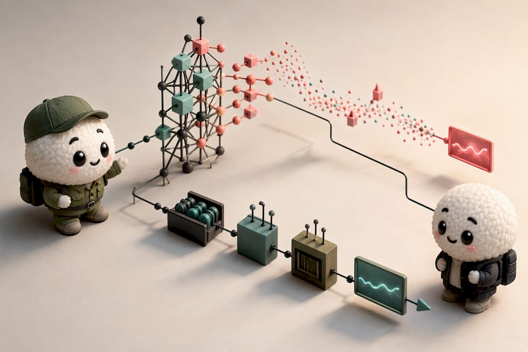
Market intelligence platforms scan numerous noisy public data streams daily to surface early market signals, and the lesson that keeps repeating is that post-processing discipline, not model sophistication, decides whether a detection pipeline earns trust. A short-window forecast with adaptive thresholding, backed by a light ensemble of reconstruction and isolation scores, catches most operationally relevant anomalies without drowning anyone in false alarms.
A 48-hour checklist worth running before committing to anything more elaborate: run a statistical baseline first; train a small LSTM or autoencoder on the same data and compare; swap a static threshold for a dynamic one and measure the false-positive drop; then triage a week of alerts manually before automating the response. If you want to see this kind of signal detection applied to live markets rather than sensor telemetry, Ontherice's AI opportunity signals run on the same underlying logic. For deeper technical grounding on interpreting model outputs, the explainable forecasting piece is worth a read before your next deployment.
— Aidil
Sources
- Dive into Time-Series Anomaly Detection: A Decade Review
- Time-Series Anomaly Detection: Overview and New Trends (VLDB tutorial)
- Detecting spacecraft anomalies using LSTMs and nonparametric dynamic thresholding (MIT thesis / supporting work)
- Generative and forecasting approaches for anomaly detection (Berkeley thesis excerpt)