

When two series both trend upward over time, their correlation tells you almost nothing about whether one drives the other. The practical rule is this: focus on transitions and explicit identification assumptions, not raw correlations. Check whether consecutive changes correlate, and then test whether past values of X improve forecasts of Y. If the answer is yes, you have a candidate causal signal worth investigating further. If the relationship disappears after differencing, you likely had a shared trend confound, not a causal relationship.
Three checks to run before anything else:
- Visual check: plot both series in levels and look for a shared monotonic trend. If both rise or fall together over time, suspect confounding by time itself.
- First-differences correlation: compute ΔX and ΔY (consecutive changes) and correlate those. A correlation that survives differencing is more credible than one computed on raw levels.
- Granger causality test: run a Granger causality test on the stationary (differenced or detrended) series to check whether past values of X add predictive power for Y beyond Y's own history.
One caveat applies throughout: observational signals, however well-constructed, are hypotheses. High-stakes decisions warrant experimental or quasi-experimental validation before acting on a causal claim.
Pro Tip: Label every series with its time unit and sampling frequency before any analysis. A monthly series and a weekly series aligned by index rather than calendar date will produce spurious lags and misleading Granger results.
Key takeaways
Causality in trend analysis requires explicit identification assumptions, transition-based checks, and method selection matched to the causal question, not just a high correlation between trending series.
| Point | Details |
|---|---|
| Prefer transitions over levels | Compute rTransitions (ΔX vs ΔY) before drawing any causal conclusion from trending series. |
| State identification assumptions | Document temporal ordering, confounders, and SUTVA before estimating any causal effect. |
| Match method to question | Use Granger for forecasting checks, ITS/CausalImpact for single interventions, DiD or synthetic control for comparative claims, DoWhy/econML for structural effects. |
| Run robustness checks | Placebo tests, permutation tests, and sensitivity to window length are the minimum standard for a credible result. |
| Ontherice for signal discovery | Use Ontherice to surface candidate causal signals and prioritise which trends warrant formal causal testing. |
Table of Contents
- What does causality in trend analysis actually mean?
- Common mistakes when inferring causality from trending data
- Which methods handle trends when you need causal estimates?
- A step-by-step workflow for causal claims in trending data
- Which software libraries should UK analysts use?
- How do you test whether your causal result is real?
- What does the research say about trends and causal judgement?
- When should you accept an observational causal claim, and when insist on an experiment?
- Ontherice surfaces the signals your causal tests need to investigate
- Sources
What does causality in trend analysis actually mean?
Causality in trend analysis is the attempt to determine whether changes in one variable produce changes in another, when both variables are observed over time and may share a common temporal trajectory. The distinction from correlation is not subtle: two series can correlate at 0.95 simply because both trend upward over a decade, with no direct relationship between them whatsoever.
The vocabulary that matters here:
- rStates vs rTransitions: rStates is the correlation between the absolute levels of X and Y. rTransitions is the correlation between their consecutive changes (ΔX and ΔY). When a linear trend is present, rStates is inflated; rTransitions controls for that trend and reflects genuine co-movement.
- Stationarity: a series is stationary when its mean, variance, and autocorrelation structure do not change over time. Most causal tests assume stationarity; trending series violate this assumption.
- First differences: subtracting each observation from the previous one. This removes a linear trend and is the simplest detrending step before running causal tests.
- Structural causal model (SCM): a formal graph-based representation of causal relationships, using directed acyclic graphs (DAGs) to encode which variables cause which, and what assumptions are required.
- Treatment vs ongoing trend: an intervention (a policy change, a product launch) is a discrete event; an ongoing trend is a gradual drift. Conflating the two is one of the most common errors in applied analysis.
Consider a simple example: monthly data show that both prescription pain-relief use and reported chronic pain scores rise over a three-year period. The rStates correlation is high. But when you compute rTransitions, the month-to-month changes in prescriptions do not reliably precede changes in pain scores. The shared trend was driven by an ageing population and changing reporting standards, not by a direct causal link in either direction.
Experimental evidence from Soo and Rottman confirms that people infer causal strength more accurately when they attend to transitions rather than levels, and that static graphs reduce accuracy compared with animated or trial-by-trial presentations.

Pro Tip: When briefing stakeholders, show the differenced series alongside the raw levels. The visual contrast alone often communicates why the raw correlation is misleading.
Common mistakes when inferring causality from trending data
Most errors in causal inference from trends share a common root: treating statistical association in levels as evidence of a causal relationship. The Australian Bureau of Statistics is direct on this point: correlation does not imply causation, and controlled studies remain the most reliable route to establishing causal claims. Observational data, however rich, guides hypothesis formation rather than confirming causal mechanisms.
The specific mistakes worth guarding against:
- Correlating levels without detrending. If X and Y both trend upward, their Pearson correlation will be high regardless of any causal link. Time acts as a lurking variable. Always check whether the correlation survives differencing or detrending before drawing any conclusion.
- Skipping stationarity tests. Running a Granger causality test on non-stationary series produces unreliable results. Augmented Dickey-Fuller (ADF) and KPSS tests take minutes to run and should precede any causal test on time-series data.
- Ignoring seasonality and structural breaks. A retail sales series with strong Christmas peaks will show spurious correlations with any other seasonal series. Decompose the series first; test for structural breaks using Chow tests or CUSUM diagnostics.
- Treating Granger tests as proof of causation. Granger causality measures predictive utility: whether past X improves forecasts of Y. It does not establish a structural causal mechanism. Analysts who present a significant Granger result as "X causes Y" are overstating the evidence.
- Relying on static visualisations. A static scatter plot of X against Y in levels hides the temporal structure entirely. Transition plots (ΔX against ΔY) and animated time-series views reveal whether co-movement happens at the right lags and in the right direction.
- Omitting placebo and permutation tests. A result that looks significant may simply reflect the method's sensitivity to the chosen window or lag structure. Running the same analysis on a placebo outcome (one that should not be affected) or on randomly permuted data gives you a baseline for comparison.
- Leaving identification assumptions undocumented. If you cannot write down the assumptions your causal claim rests on, you cannot defend it. Temporal ordering, absence of simultaneous confounders, and stable unit treatment value (SUTVA) are the minimum to state explicitly.
Which methods handle trends when you need causal estimates?
No single method suits every causal question in trending data. The choice depends on whether you have an intervention, a control group, a long pre-period, or only observational series. Below is a structured overview of the main approaches, followed by the assumptions each one requires.
Method overview
Granger causality is a forecasting check, not a causal proof. It tests whether lagged values of X improve predictions of Y in a VAR (vector autoregression) model. Requires stationary series; difference or detrend first. Useful for exploratory screening and for supporting (not confirming) causal hypotheses. Implemented in Python via statsmodels.tsa.stattools.grangercausalitytests.
Interrupted time series (ITS) and CausalImpact suit single-intervention problems where you have a clear before/after break. CausalImpact (Google's R package, with a Python port) builds a Bayesian structural time-series model on the pre-intervention period and projects a counterfactual forward. The gap between the counterfactual and the observed post-intervention series is the estimated causal effect. Requires a reasonably long pre-period (typically 30+ observations) and the assumption that the pre-intervention trend would have continued absent the intervention.
Difference-in-differences (DiD) compares the change in an outcome for a treated group against the change for a control group over the same period. The key assumption is parallel trends: in the absence of treatment, both groups would have followed the same trajectory. Pre-trend tests (checking that the groups moved in parallel before the intervention) are mandatory. Implemented in Python via statsmodels or linearmodels.
Synthetic control constructs a weighted combination of donor units to match the pre-intervention trajectory of the treated unit, then uses the post-intervention divergence as the causal estimate. Well-suited when there is only one treated unit (a country, a region, a product) and several plausible donor comparators. Requires a long pre-period for good donor-pool fit.
Structural causal models (SCMs) and causal ML use DAGs to encode domain knowledge about causal structure, then estimate effects from data under those assumptions. DoWhy (Microsoft's Python framework) provides a four-step API: model, identify, estimate, refute. econML extends this with heterogeneous treatment effect estimators (double ML, causal forests) suited to high-dimensional observational data. Both are available via pip and work within standard UK Python environments.
Econometric differencing and ARIMA adjustments remove trends parametrically before estimation. ARIMA models (available in statsmodels.tsa.arima.model) handle non-stationarity through the integrated (I) component. Useful when the goal is to model the trend-adjusted relationship between series rather than estimate a discrete intervention effect.
Comparison at a glance
| Method | When to use | Core assumptions | Data requirements | Key strength / limitation |
|---|---|---|---|---|
| Granger causality | Exploratory forecasting check | Stationarity, correct lag order | Moderate length (50+ obs) | Fast; does not prove causation |
| ITS / CausalImpact | Single clear intervention | Trend continuity counterfactual | 30+ pre-intervention obs | Handles non-stationarity; single treated unit only |
| Difference-in-differences | Comparative pre/post with control | Parallel pre-trends | Two groups, pre and post data | Credible with good control; fails if trends diverge |
| Synthetic control | One treated unit, multiple donors | Good donor-pool pre-period fit | Long pre-period, donor pool | Strong counterfactual; sensitive to donor selection |
| SCMs / DoWhy / econML | Structural or heterogeneous effects | DAG correctness, no hidden confounders | Varies; multivariate | Explicit assumptions; computationally intensive |
| ARIMA / differencing | Detrending before regression | Correct ARIMA order | Moderate length | Simple; removes trend but not all confounds |
Assumptions every analyst must confirm before proceeding: temporal ordering (X precedes Y), no simultaneous unmeasured confounders, SUTVA where applicable, and correct detrending or stationarity transformation.
Pro Tip: Consider coupling trend modelling with residual modelling as an advanced pattern. Architectures that use the estimated trend state as a contextual prior for residual modelling, as in the CTMNet approach, tend to produce more robust forecasts under changing regimes than models that treat trend and residual as independent components.
A step-by-step workflow for causal claims in trending data
This sequence takes you from a raw series to a defensible causal estimate. Run it in order; skipping steps is where most errors enter.
- Clarify the causal question and target estimand. Write one sentence: "Does X cause Y, and by how much, for which units, over what time horizon?" Vague questions produce vague answers.
- Draw a DAG. Sketch the assumed causal graph on paper or in Dagitty. Identify confounders, mediators, and colliders. This forces you to state your assumptions before touching the data.
- Visualise raw series in levels. Plot X and Y on the same axis. Note shared trends, seasonality, and any obvious structural breaks. This is the rStates view.
- Compute and plot first differences. Plot ΔX and ΔY. Compute their correlation. A relationship that appears only in levels but not in differences is almost certainly a shared-trend artefact.
- Test stationarity. Run ADF and KPSS tests on both the raw series and the differenced series. Confirm the order of integration before proceeding.
- Check for seasonality and structural breaks. Use seasonal decomposition (STL or classical) and Chow or CUSUM tests. Document any breaks and decide whether to model them explicitly.
- Choose and justify your detrending approach. First differencing is the default for I(1) series. Seasonal differencing handles periodic patterns. Parametric detrending (fitting and removing a trend line) is an alternative but introduces model dependence. State your choice and why.
- Select your method and run the primary estimate. Match the method to the question using the comparison above. For a single intervention, use ITS or CausalImpact. For a comparative claim, use DiD or synthetic control. For structural claims, use DoWhy or econML.
- Run robustness checks. Placebo interventions, permutation tests, and sensitivity to window length are the minimum. See the validation section below for the full list.
- Document assumptions and limitations. Write them down. Every causal claim rests on assumptions that could be wrong; stating them is what separates analysis from advocacy.
Diagnostic checks at each stage: ADF/KPSS p-values at step 5; autocorrelation function (ACF) and partial ACF plots at step 6; pre-trend tests and balance checks for DiD at step 8; donor-pool fit plots for synthetic control at step 8.
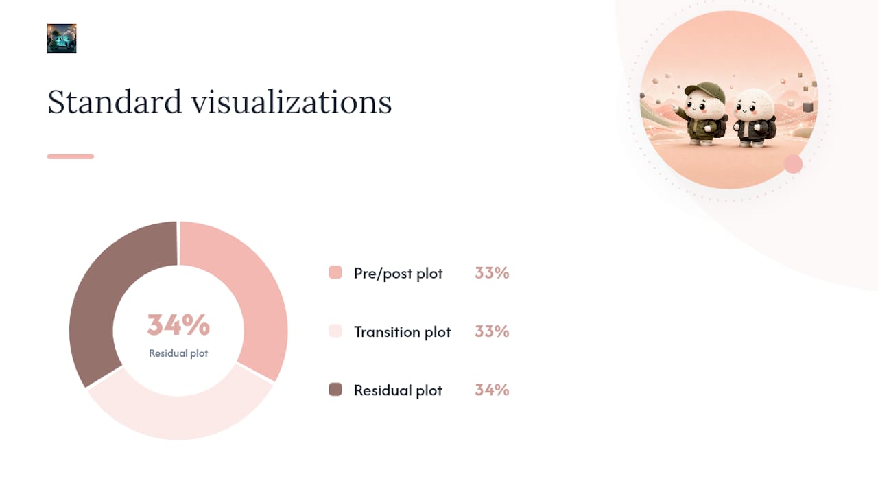
For visualisation, produce three plots as standard: a pre/post plot with counterfactual bands, a transition plot (ΔX against ΔY), and a residual plot after trend removal. For stakeholder communication, an animated version of the transition plot, showing how the relationship evolves observation by observation, is often more persuasive than any static chart.
Pro Tip: For short series (fewer than 50 observations), Granger tests and DiD estimates become unreliable. In that case, lean on synthetic control with a well-matched donor pool, or use a Bayesian structural model (CausalImpact) that can borrow strength from the prior. Document the limitation explicitly.
Which software libraries should UK analysts use?
All libraries listed here are freely available in standard Python and R environments, with no UK-specific licensing restrictions. Installation via pip or CRAN is straightforward on any major operating system.
- DoWhy (Python, Microsoft / PyWhy): the most complete SCM framework for applied analysts. Its four-step API (model, identify, estimate, refute) enforces explicit assumption documentation. The
refute_estimatemethods include placebo and data-subset robustness checks out of the box. - econML (Python, Microsoft): causal ML estimators including double ML, causal forests, and instrumental variable methods. Best suited to high-dimensional observational data where treatment effect heterogeneity matters.
- CausalImpact (R package by Google; Python port
causalimpactvia pip): Bayesian structural time-series for single-intervention analysis. The R version is the most mature; the Python port covers the core use case. Both handle non-stationary series and produce credible-interval counterfactual bands. - statsmodels (Python): covers Granger causality tests (
grangercausalitytests), ARIMA and SARIMAX modelling, ADF/KPSS stationarity tests, and VAR models. The go-to library for time-series econometrics in Python. - scikit-learn (Python): not a causal library, but essential for pre-processing, feature engineering, and building the ML components that feed into econML pipelines.
- Synthetic control packages:
pysynconandSynthControlin Python;Synthin R. All handle the donor-pool optimisation and produce pre/post fit diagnostics.
For a practical comparison of AI-assisted platforms that can surface candidate signals before you run formal causal tests, the AI tools available on Ontherice provide a useful starting point for exploratory hypothesis generation.
Pro Tip: Pin your library versions in a requirements.txt or renv.lock file before sharing any analysis. Causal estimates from DoWhy and econML can shift between minor versions as default estimators change. Reproducibility is part of the causal claim.
How do you test whether your causal result is real?
A single significant result from a single method is not enough. The robustness checks below are the minimum standard for a credible causal claim in trend data.
- Placebo intervention: apply your method to a date or unit where no intervention occurred. If you find a significant effect there too, your method is picking up noise or a systematic pattern, not a causal signal.
- Permutation test: randomly shuffle the treatment assignment (or the intervention date) many times and recompute the effect estimate each time. Your observed effect should sit in the tail of this null distribution.
- Varying the pre/post window: re-run the analysis with shorter and longer pre-intervention periods. A genuine effect should be stable; an artefact will fluctuate with window choice.
- Falsification outcomes: test the method on an outcome that should not be affected by the intervention. A significant result on a falsification outcome is a red flag.
- Lagged-effect specifications: try different lag structures. If the effect only appears at one very specific lag and disappears at adjacent lags, treat that with scepticism.
- Sensitivity to detrending method: compare results under first differencing, seasonal decomposition, and parametric detrending. Divergent results across methods signal that the causal estimate is sensitive to modelling choices that should be justified, not assumed.
For diagnostic output, inspect residual autocorrelation after estimation (a Ljung-Box test on residuals), compare in-sample fit with out-of-sample forecast performance, and use Granger tests as supporting evidence for predictiveness rather than as standalone causal proof.
On effect sizes: in trend contexts, a causal effect is most interpretable as a change in the rate of change rather than a level shift. Report the estimated effect in units of ΔY per unit ΔX, with bootstrapped confidence intervals. A wide interval on a small effect is an honest result; a narrow interval on a large effect from a short series should prompt scepticism about model assumptions.
For ADF and KPSS tests, report the test statistic and p-value but avoid treating a p-value of 0.049 as categorically different from 0.051. The tests have known size distortions in small samples; use them as one input among several, not as a mechanical gate.
What does the research say about trends and causal judgement?
Two bodies of evidence directly motivate the practical rules in this guide.
The first comes from Soo and Rottman's experimental work on how people learn causal relationships from time-series graphs. Their experiments show that when a shared linear trend is present, participants systematically overestimate causal strength when they attend to the levels of the series (rStates). Accuracy improves substantially when participants attend to transitions (rTransitions, the correlation between consecutive changes). Critically, the presentation format matters: animated or trial-by-trial displays, which make transitions salient, produce better causal judgements than static graphs of the full series.
The practical implication is not just about human cognition. It is a design principle for analysis: build your primary diagnostic around rTransitions, and present results in formats that make the transition structure visible.
The second body of evidence concerns model architecture. A coupled decomposition architecture (CTMNet), published in Scientific Reports, encodes trend causally using a unidirectional trend encoder and then uses the trend state to modulate residual features adaptively. Tested across 10 real-world multivariate time-series benchmarks, this approach achieves competitive or leading forecasting performance. The key insight is that treating trend and residual as independent components, as most classical decomposition methods do, discards information. The trend state is a contextual prior for the residual; modelling that interaction explicitly produces more robust forecasts under regime changes.
Practical implementation notes:
- Prefer first differencing when the trend is approximately linear and the series is long enough for the differenced series to retain adequate power.
- Use parametric detrending (fitting a polynomial or spline trend and removing it) when the trend is nonlinear and the pre-period is long.
- Consider coupled trend-residual architectures when the goal is forecasting under non-stationarity rather than estimating a discrete intervention effect.
When documenting an analysis, citing Soo and Rottman alongside your transition-based checks, and CTMNet alongside any coupled modelling choices, strengthens methodological credibility with technically literate reviewers.
Pro Tip: When presenting to a mixed audience, show a side-by-side of the static levels plot and the animated transition plot. The contrast is usually enough to make the rStates vs rTransitions distinction intuitive without any algebra.
When should you accept an observational causal claim, and when insist on an experiment?
The honest answer is that observational causal claims are almost always provisional. The standard conditions for inferring causation require temporal sequencing, a non-spurious relationship, and the elimination of alternative explanations. In practice, eliminating all alternatives from observational data alone is rarely possible.
The pragmatic trade-off is between speed and certainty. Observational methods, run well with explicit assumptions and robust checks, are genuinely useful for early signals and for forecasting. They are the right tool when an experiment is infeasible, when the decision is low-stakes, or when you need to prioritise which hypotheses are worth testing further. A well-executed DiD or synthetic control analysis can be highly credible when the parallel-trends assumption holds and the robustness checks pass.
But for high-stakes decisions, the bar should be higher. If the decision involves significant resource allocation, a regulatory submission, or a public claim about what causes what, push for an A/B test, a phased rollout with a holdout group, or a commissioned synthetic-control evaluation with independent replication. The cost of a wrong causal claim in those contexts almost always exceeds the cost of running a proper experiment.
One underappreciated middle ground: a pre-registered observational analysis. Committing to your DAG, your estimand, your method, and your robustness checks before seeing the outcome data substantially strengthens the credibility of an observational result. It does not make the claim experimental, but it removes the most common source of scepticism, which is that the analyst chose the method after seeing which one gave the desired answer.
Document every decision. Future analysts, auditors, and stakeholders need to understand not just what you found but what assumptions you made and what you would have concluded if those assumptions had been different.
Ontherice surfaces the signals your causal tests need to investigate
The hardest part of causal analysis in trend data is often not the estimation. It is knowing which signals are worth testing in the first place. Ontherice scans global market data continuously, surfaces early-stage trend signals across finance, technology, crypto, and consumer sectors, and ranks them by momentum before they reach mainstream awareness.

For analysts, that means a shorter path from "something is moving" to "here is a testable causal hypothesis." The platform's AI engines extract signals from noisy data and present them with transparent scoring, so you can prioritise which emerging patterns deserve a formal DiD, CausalImpact, or DoWhy analysis rather than spending weeks on exploratory data work. Signals from Ontherice are hypotheses, not conclusions: they tell you where to look, not what causes what. The causal identification and validation work remains yours to do. Start with the AI Opportunities feed to see which signals are gaining traction right now.
Sources
- CTMNet: causal trend evolution and adaptive modulation for time series forecasting | Scientific Reports
- Distinguishing causation and correlation_ Causal learning from time-series graphs with trends
- Correlation and causation | Australian Bureau of Statistics
- Correlation vs. Causation: What’s the Difference? | Coursera
- Granger causality