Spot Early Trends: Topic Clustering for Analysts SBERT UMAP HDBSCAN

Topic clustering analysis groups documents by shared meaning rather than shared vocabulary, using vector embeddings and unsupervised algorithms to surface themes without predefined categories. For short or noisy text, an embedding-based pipeline (SBERT into UMAP into HDBSCAN) beats classical methods almost every time. For long, well-structured documents, LDA or NMF still holds up. The two catches: embedding pipelines need more compute, and most methods force one topic per document even when text covers several.

TL;DR:

Embedding-based clustering methods outperform classical models on short or noisy texts but require higher computational resources.

Use hard clustering for single-topic, short documents, and probabilistic models for long, multi-theme texts to accurately reflect document content.

Proper dimensionality reduction (like UMAP) is essential before clustering to prevent high-dimensional distance distortions.

Incorporate human validation by reviewing a sample of documents per cluster and adjust parameters to ensure meaningful groupings.

Emerging techniques combine joint learning and LLM labeling to generate more coherent, readable topics while handling evolving, streaming data.

What topic clustering analysis actually measures
Algorithm families: from LDA to embedding-driven pipelines
Building a topic clustering pipeline step by step
How to check if your clusters actually mean something
Matching the method to your data and budget
Python and R tools for building your own pipeline
Where topic clustering analysis goes wrong
What's next: joint learning, LLM labelling, and streaming clusters.
A practical note on using clustering to spot early trends
Getting managed topic signals without building the pipeline yourself
Sources

What topic clustering analysis actually measures

Topic clustering analysis sorts a corpus into groups of documents that discuss the same underlying subject, then lets you inspect each group to work out what it's about. That's the whole job: partition first, interpret second. It sits next to, but is not identical to, classical topic modelling, and the distinction trips up a lot of people who use the terms interchangeably.

Rice-ball mascots studying document clusters on panel

Clustering produces hard partitions. Every document lands in exactly one group (or gets marked as noise, depending on the algorithm), and there's no numerical answer to "how much" a document belongs to a cluster beyond distance to a centroid or density. Probabilistic topic models such as Latent Dirichlet Allocation work differently: they assume every document is a mixture of topics in different proportions, and they hand you a probability distribution rather than a label. Under a clustering approach, it just gets assigned to whichever cluster centroid it sits closest to.

Which framing you want depends on what the documents actually look like:

Choose hard clustering when documents are typically single-topic, short, or you need a clean, browsable taxonomy for navigation or tagging.
Choose probabilistic topic modelling when documents routinely blend several themes, such as long reports, policy documents, or academic papers.
Choose a hybrid view (cluster first, then inspect soft membership scores) when you need the simplicity of clusters for reporting but still want to catch documents that don't fit cleanly anywhere.

The practical test: pull ten random documents from your corpus and ask whether a human would confidently give each one a single label. If yes, clustering is the right lens. If most documents need two or three labels to describe fairly, you're dealing with a mixed-membership problem, and forcing a hard partition on it will quietly throw away information.

Algorithm families: from LDA to embedding-driven pipelines

Four broad families dominate practice, and each one makes a different bet about what "similarity" means.

Classical probabilistic models — LDA and Non-negative Matrix Factorisation (NMF) — treat documents as bags of words and infer topics from co-occurrence patterns. LDA assumes a generative process where documents are drawn from a mixture of topics and topics are distributions over words; NMF factorises the document-term matrix directly into two lower-rank matrices. Both work well on long, structured text with a large, consistent vocabulary; both struggle on tweets, chat logs, or product reviews where sparse word overlap gives them almost nothing to latch onto. The University of Pennsylvania's topic modelling guide lays out a workable sequence for either: preprocess, build the document-term matrix, run the model, then interpret and retune the topic count based on how coherent the outputs look.

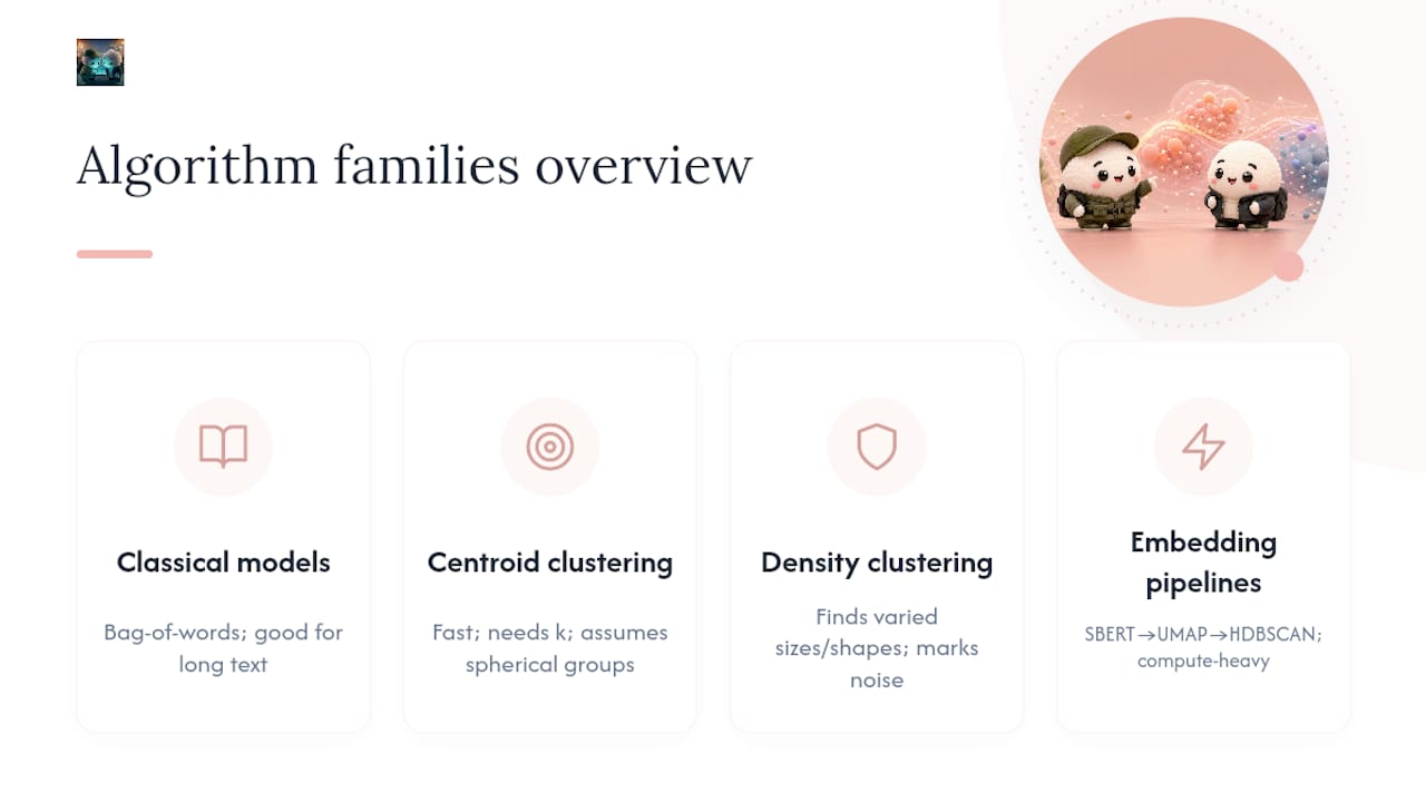
Comparison diagram of four topic clustering algorithm families

Centroid-based clustering — k-means and hierarchical (agglomerative) clustering — groups points by proximity to a centre or by iteratively merging nearest neighbours. Fast and simple, but k-means forces you to pick the number of clusters upfront and assumes roughly spherical, evenly sized groups, which real topic distributions rarely are.

Density-based clustering — DBSCAN and its hierarchical successor HDBSCAN — groups points by local density instead of distance to a fixed centre. This matters enormously for topic work because it does two things centroid methods can't: it finds clusters of wildly different sizes and shapes, and it explicitly labels outliers as noise rather than cramming them into the nearest group. A rare but genuine topic with fifteen documents won't get diluted into a giant catch-all cluster.

Embedding-driven pipelines — BERTopic, Top2Vec, and TopiCLEAR — represent the current default for anyone working with modern language data. Instead of word counts, they encode each document as a dense semantic vector using a transformer model, then cluster the vectors. BERTopic's approach runs SBERT embeddings through UMAP for dimensionality reduction, clusters the reduced vectors with HDBSCAN, and generates topic representations using a class-based TF-IDF variant, reporting results competitive with classical models across multiple benchmarks. Top2Vec follows a similar embed-then-cluster logic with its own representation step. TopiCLEAR takes it further, pairing SBERT embeddings with a Gaussian Mixture Model and an adaptive projection step that iteratively refines the clusters, and reported higher Adjusted Rand Index and Adjusted Mutual Information scores than several baselines on short-text datasets including 20News and TweetTopic, without requiring heavy preprocessing.

The trade-off is compute. Embedding methods need a transformer model to encode every document, which costs more time and memory than counting word frequencies. Classical models remain faster and cheaper on large, well-behaved corpora where semantic nuance matters less than raw throughput.

Building a topic clustering pipeline step by step

Here's the sequence that holds up in practice, from raw text to labelled clusters you'd actually show a stakeholder.

Minimal preprocessing. Embedding models are trained on natural language, so aggressive stemming or stopword stripping usually hurts more than it helps. Lowercase, strip boilerplate (headers, signatures, HTML), and leave the rest to the model. Classical pipelines still need tokenisation, stopword removal, and often lemmatisation.
Pick an embedding model. Sentence-transformers (SBERT) is the standard choice for general text. Fine-tune on domain-specific data (legal, medical, financial) only if a generic model's clusters look muddled on a validation sample. Off-the-shelf SBERT is usually good enough to start.
Reduce dimensionality before clustering. High-dimensional embeddings (384 to 1,024 dimensions is typical) make distance metrics behave strangely. UMAP preserves both local and global structure better than PCA or t-SNE for this kind of transformer embedding and tends to improve both clustering accuracy and runtime. Use PCA instead when you need a fast, deterministic reduction and interpretability of components matters more than cluster quality.
Cluster the reduced embeddings. HDBSCAN is the default because it doesn't require you to guess the number of clusters and it handles noise gracefully. Start min_cluster_size at roughly 1% of your corpus size and adjust from there; smaller values create many niche clusters, larger values force broader groupings. If you need every document assigned (no noise bucket) and roughly know the topic count, k-means is a reasonable fallback.
Extract topic representations. Class-based TF-IDF (the method behind BERTopic) treats each cluster as a single document and scores words by how distinctive they are to that cluster versus the rest of the corpus. Centroid-word extraction (nearest words to the cluster centre in embedding space) is a quick alternative. For genuinely readable output, feed each cluster's top documents to an LLM and ask for a short summary label.
Validate with humans before shipping. Pull five to ten representative documents per cluster and read them. If the topic doesn't hold together on a manual read, adjust min_cluster_size or revisit the embedding choice rather than trusting the automated label blindly.

Pro Tip: Run the same pipeline three times with different random seeds at the embedding and clustering stages. If cluster boundaries shift dramatically between runs, your parameters are producing brittle results, not real structure.

How to check if your clusters actually mean something

Numbers alone won't tell you whether a topic model is good. A peer-reviewed evaluation of clustering and topic modelling methods over health-related social media text found measurable performance differences across methods and specifically recommended pairing automated metrics with human judgement, because neither alone gives a reliable picture.

The automated toolkit splits into two camps:

Coherence metrics (NPMI, c-v) measure whether the top words in a topic tend to co-occur in real documents. High coherence means the topic's keywords make semantic sense together.
Clustering-agreement metrics (Adjusted Rand Index, Adjusted Mutual Information) compare your clustering against a ground-truth labelling, when one exists, and correct for chance agreement.
Silhouette score measures how well-separated clusters are in embedding space, without needing any ground truth at all.
Exclusivity checks whether a topic's top words are unique to it or bleeding into neighbouring topics, a common failure mode when the topic count is set too high.

TopiCLEAR's authors reported higher ARI and AMI scores than several baseline methods across four short-text benchmark datasets, which is a useful sanity check for how much headroom modern embedding approaches have over older baselines on messy text.

Metrics can still mislead you. Coherence scores reward tight, narrow topics, so a model can score well while producing forty near-duplicate micro-topics that no human would find useful. Silhouette scores get distorted by noise points if you're using HDBSCAN. The fix is procedural, not statistical: run an intrusion test, where you insert one out-of-place word into a topic's keyword list and ask a colleague to spot the intruder. If they can't, your topic isn't distinctive enough regardless of what the coherence score says. Also track cluster size distribution and re-run with different seeds; a cluster that vanishes or merges under a seed change was never stable to begin with.

Matching the method to your data and budget

The single biggest predictor of which method will work is text length and structure, not the size of your dataset.

Short, noisy, or colloquial text (tweets, support tickets, chat transcripts) favours embedding-based pipelines. Word co-occurrence, which LDA and NMF depend on, breaks down when documents are only a sentence or two long, but embeddings capture meaning from context even in short spans.
Long, structured corpora (academic papers, legal filings, formal reports) still play to LDA and NMF's strengths, and they run considerably faster at scale because there's no transformer inference step involved.
Multilingual corpora generally favour embedding approaches too, since multilingual SBERT variants map semantically similar text across languages into nearby vector space, something bag-of-words methods can't do at all.

Compute constraints matter as much as data type. Encoding millions of documents through a transformer model without a GPU will crawl. If you're working at that scale without dedicated hardware, either sample down to a representative subset for model development and apply the fitted pipeline to the rest, or accept the speed of LDA/NMF as the trade-off for feasibility.

On hard versus soft assignment: default to soft (probabilistic) membership whenever documents plausibly cover multiple themes, and reserve hard clustering for genuinely single-topic inputs like short reviews or ticket subjects.

Pro Tip: If you're not sure which family fits, run both a quick LDA pass and a quick BERTopic pass on a 500-document sample. The one that produces topics you can name in under ten seconds each is the one to build out.

Python and R tools for building your own pipeline

The Python ecosystem covers this workflow end to end. Sentence-transformers provides SBERT embeddings out of the box. BERTopic wraps the full embed-reduce-cluster-represent pipeline into a single package and is the fastest route to a working prototype. Top2Vec offers a comparable embedding-based alternative with a slightly different topic-representation approach. umap-learn and hdbscan are the standalone libraries behind BERTopic's reduction and clustering steps, useful if you want to swap in a custom clustering algorithm. scikit-learn covers k-means, agglomerative clustering, NMF, and most evaluation metrics. Gensim remains the standard for LDA if you're staying with a classical approach.

Rice-ball mascots exploring AI tool components in lab

R users aren't left out: topicmodels and stm (Structural Topic Model) cover LDA-style workflows with strong support for including document metadata as covariates, and text2vec handles vectorisation and clustering pipelines natively in R. For quick, no-code exploration before committing to a pipeline, browser-based tools like Voyant let you eyeball word frequencies and co-occurrence patterns on a small corpus.

Reference implementations for the newer research are publicly available, with GitHub repositories accompanying both the BERTopic paper and the TopiCLEAR paper, which is worth checking before you rebuild something from scratch.

A few habits pay off later: fix random seeds at the embedding, UMAP, and clustering stages so results are reproducible; record which model version and reduction parameters produced a given result; and keep a fixed evaluation split separate from the data you use to tune parameters, so your coherence scores aren't quietly overfit to the same documents you eyeballed while adjusting min_cluster_size.

Where topic clustering analysis goes wrong

The most common failure isn't a bad algorithm choice, it's skipping dimensionality reduction. Feeding raw 768-dimensional embeddings straight into a clustering algorithm degrades distance metrics badly, because in high-dimensional space nearly every point ends up roughly equidistant from every other point. UMAP or PCA aren't optional polish; they're what makes the clustering step work at all.

Labelling by top keywords alone is the second big trap. A cluster's top five TF-IDF words might all technically belong, while completely missing the thread a human reader would actually notice on reading the documents. Combining keyword extraction with LLM-generated summaries closes that gap, but only if you calibrate it: always show the LLM several exemplar documents per cluster, not just the keyword list, and spot-check a sample of labels against the source text to catch hallucinated themes before they ship.

Parameter tuning cuts both ways. Too aggressive a min_cluster_size or too high a target topic count fragments a single coherent theme into five near-identical clusters, an over-segmentation problem that inflates your topic count without adding insight. Too conservative, and distinct themes get smothered into one oversized catch-all cluster.

Multi-topic documents deserve specific attention, since most clustering pipelines force one label per document. Where that's a problem, inspect soft membership proxies (distance to the second-nearest cluster centre, for instance) or switch to a probabilistic model that reports mixed membership honestly.

Finally, document your decisions. Note which embedding model, reduction parameters, and cluster count you settled on, and why, so a stakeholder questioning a topic label six months later gets an answer grounded in a decision, not a guess.

Pro Tip: Keep a running log of "borderline" documents, ones that sat near a cluster boundary during validation. They're often the first sign a topic needs splitting or a parameter needs revisiting.

What's next: joint learning, LLM labelling, and streaming clusters.

The frontier of topic clustering analysis is moving away from the simple embed-then-cluster recipe towards models that learn the representation and the clustering jointly. TopClus trains a spherical latent space with a fixed number of soft clusters while simultaneously modelling topic-word and document-topic distributions, producing topics that read as more coherent and distinctive than a naive UMAP-plus-clustering pass, because the projection itself is optimised for topic separability rather than borrowed from a general-purpose dimensionality reduction step. TopiCLEAR pushes a related idea with its adaptive projection, refining cluster assignments iteratively rather than clustering once and stopping.

LLM-guided labelling is the other major shift. Instead of reading off top keywords, you prompt a language model with a cluster's representative documents and ask it to summarise the shared theme. This produces genuinely readable labels for non-technical stakeholders, but it introduces its own risks: inconsistent granularity between clusters, and occasional hallucinated labels that sound plausible but don't match the underlying documents. The fix, again, is to always ground the prompt in real exemplar documents rather than keyword lists alone.

Streaming and online clustering is the practical concern for anyone tracking topics over time rather than analysing a static corpus. Static clustering assumes your topics are fixed; real corpora drift as new themes emerge and old ones fade. Worth testing directly: run an A/B comparison between LDA and BERTopic on the same corpus and compare coherence and human-readability side by side, and separately compare LLM-generated labels against c-TF-IDF keyword labels on the same clusters to see which stakeholders actually find clearer.

A practical note on using clustering to spot early trends

The most useful thing clustering has taught anyone who watches emerging markets: a rising theme rarely announces itself with obvious keywords. It shows up first as a small, oddly dense group of documents that don't cleanly match any existing category, exactly the kind of signal HDBSCAN is built to surface rather than bury in a larger cluster. Catching that early is the entire point of running clustering over noisy, fast-moving text instead of waiting for a theme to become common enough that keyword search would find it anyway.

For anyone wanting to try this without building infrastructure first, a one-day pilot works: pull a few thousand recent documents from one domain, run the SBERT-into-UMAP-into-HDBSCAN pipeline described earlier, and look specifically at the smallest stable clusters rather than the largest. The small ones are where early signals hide. Ontherice's own tutorials walk through variations of this approach for readers who want to see it applied to live market data.

— Aidil

Getting managed topic signals without building the pipeline yourself

Building the pipeline described above is entirely doable, but it takes real engineering time: embedding infrastructure, parameter tuning, ongoing revalidation as your corpus drifts. Ontherice exists for the teams who'd rather skip that build and go straight to the output. It scans public data across sectors and turns the same underlying idea, dense clusters of unusual activity, into ranked signal feeds and AI-generated summaries you can act on directly.

That's the practical difference: instead of maintaining an HDBSCAN pipeline and retuning it every time your corpus shifts, you get continuously updated rankings and topic summaries maintained on your behalf. It suits analysts and product or strategy teams who understand exactly what a good cluster looks like but don't have the engineering hours to keep one running in production. The RankingsGeneratorEngine turns that same signal-detection logic into ranked, browsable output across finance, technology, crypto, and other sectors, with transparent scoring so you can see why a topic is trending rather than taking it on faith. If you want to see what an early-stage signal looks like before it hits the mainstream, start by browsing the current rankings and see how the clustering holds up against a domain you already know well.